on
Blogpost 5: Air Campaigns
Hi everyone! Welcome back to this weeks election analytics blog post. While last week we were looking at the effect of expert prediction and polls, this week I am turning our attentions to the efficacy of air campaigns and it’s role in predicting election outcomes.
Political campaigns are extraordinary operations with thousands of people working and volunteering each year. People dedicate their lives to running and studying these campaigns. With all this attention focused on persuading others and turning out support, the question becomes: How much does the adveretising element of campaigns matter? Perhaps one of the most prominent features of campaigns and political persuasion these days are advertisements. These aired ads use technology to motivate individuals to vote for a candidate on the ballot. Traditionally, on campaigns one would believe an increase in ads would increase support for a candidate. What I’m here to investigate today is if this line of thinking is really true.
knitr::opts_chunk$set(echo = FALSE, message = FALSE, warning = FALSE)
# Loading in necessary libraries

library(tidyverse)
## ── Attaching packages ─────────────────────────────────────── tidyverse 1.3.1 ──## ✔ ggplot2 3.3.5 ✔ purrr 0.3.4
## ✔ tibble 3.1.6 ✔ dplyr 1.0.7
## ✔ tidyr 1.2.0 ✔ stringr 1.4.0
## ✔ readr 2.1.2 ✔ forcats 0.5.1## Warning: package 'tidyr' was built under R version 4.0.5## Warning: package 'readr' was built under R version 4.0.5## ── Conflicts ────────────────────────────────────────── tidyverse_conflicts() ──
## ✖ dplyr::filter() masks stats::filter()
## ✖ dplyr::lag() masks stats::lag()library(ggplot2)
library(stargazer)## Warning: package 'stargazer' was built under R version 4.0.5##
## Please cite as:## Hlavac, Marek (2022). stargazer: Well-Formatted Regression and Summary Statistics Tables.## R package version 5.2.3. https://CRAN.R-project.org/package=stargazerlibrary(janitor)##
## Attaching package: 'janitor'## The following objects are masked from 'package:stats':
##
## chisq.test, fisher.testlibrary(readxl)## Warning: package 'readxl' was built under R version 4.0.5library(tidyverse)
library(ggplot2)
library(blogdown)
library(stargazer)
library(readr)
library(usmap)## Warning: package 'usmap' was built under R version 4.0.5library(rmapshaper)## Registered S3 method overwritten by 'geojsonlint':
## method from
## print.location dplyrlibrary(sf)## Warning: package 'sf' was built under R version 4.0.5## Linking to GEOS 3.9.1, GDAL 3.4.0, PROJ 8.1.1; sf_use_s2() is TRUElibrary(janitor)
library(tigris)## Warning: package 'tigris' was built under R version 4.0.5## To enable caching of data, set `options(tigris_use_cache = TRUE)`
## in your R script or .Rprofile.library(leaflet)## Warning: package 'leaflet' was built under R version 4.0.5##BUILD DISTRICT LEVEL MODEL
##
##   2012   2014   2016   2018
## 685756 481597 470787 977127
##
## 2012 2014 2016 2018
## 685756 481597 470787 977127## # A tibble: 247,208,009 × 24
## year st_cd_fips office state.x winner_party DemCandidate DemStatus
## <dbl> <chr> <chr> <chr> <chr> <chr> <chr>
## 1 2012 0102 House Alabama R Ford, Therese Challenger
## 2 2012 0102 House Alabama R Ford, Therese Challenger
## 3 2012 0102 House Alabama R Ford, Therese Challenger
## 4 2012 0102 House Alabama R Ford, Therese Challenger
## 5 2012 0102 House Alabama R Ford, Therese Challenger
## 6 2012 0102 House Alabama R Ford, Therese Challenger
## 7 2012 0102 House Alabama R Ford, Therese Challenger
## 8 2012 0102 House Alabama R Ford, Therese Challenger
## 9 2012 0102 House Alabama R Ford, Therese Challenger
## 10 2012 0102 House Alabama R Ford, Therese Challenger
## # … with 247,207,999 more rows, and 17 more variables:
## # DemVotesMajorPercent <dbl>, winner_candidate <chr>,
## # winner_candidate_inc <chr>, president_party <chr>, dem_status <dbl>,
## # creative <chr>, race <chr>, airtime <time>, est_cost <dbl>,
## # ad_purpose <chr>, party <chr>, cycle <dbl>, station <chr>, ad_tone <chr>,
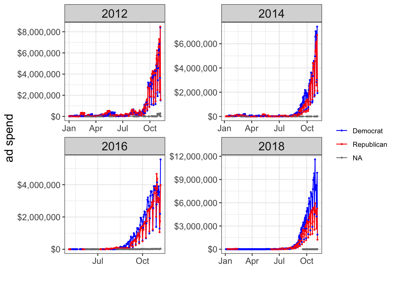
## # avg_spend <dbl>, average_support_dem <dbl>, average_support_rep <dbl>To begin this analysis, I first wanted to descriptively look total ad spend by a party in a given election cycle. Looking at the data below, you can see that in recent years, democrats are spending more than republicans closer to an election cycle. Additionally, all campaigns are trying to spend more money on ads the closer it gets to election day. Interestingly, republican ad spend has decreased overtime since 2012 while Democrats ad spend certainly hasen’t consistently.
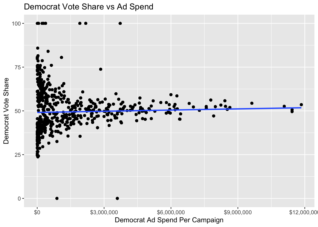
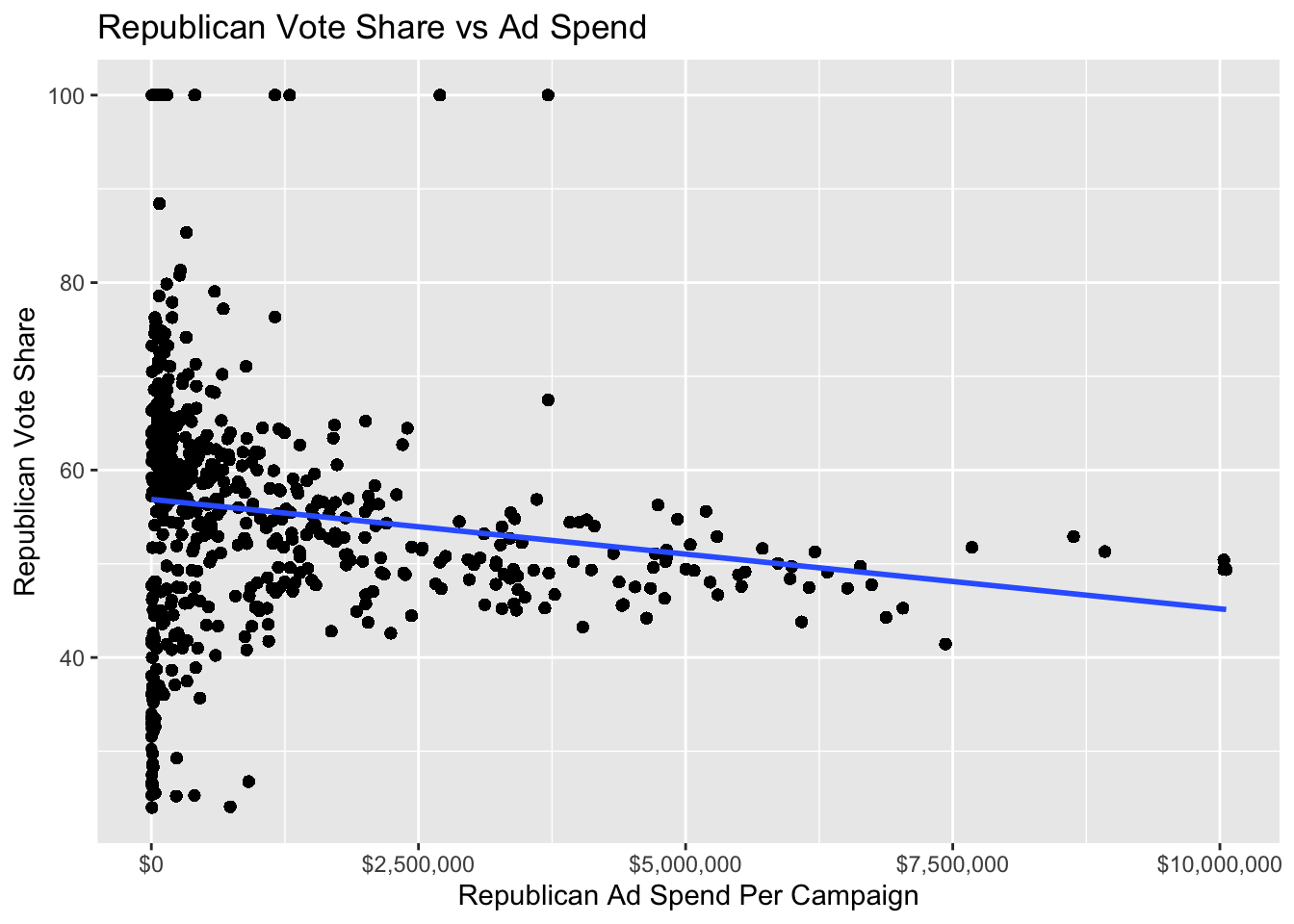
After seeing some differential ad spend between the two parties in the most recent house elections, I wanted to see if there is a visual descriptive correlation between democrat vote share and democrat ad spend. The plot of the linear relationship between a party’s total ad spend per a campaign and the party vote share is illustrated below. Looking at the plot for democrats, it appears that there is possibly a small positive correlation between ad spend and party vote share. However, this appears to be driven by an outlier point 12 million in ad spending. The relationship, if significant at all, seems very tiny especially since most of the points show little ad spend at all. This is likely due to the historical nature of the data and increasing but more recent prevalance of air campaigning. Looking at the graph of republican vote share versus total ad spend, there appears to be a negative correlation between total ad spend and party vote share. However, this seems to be driven by a few outlier points of higher spend and lower vote share. From looking at these two graphs, total ad spend by a party does not seem to clearly drive party vote share in any consistent way. This makes me think perhaps total ad spend will be a weaker covariate than I’d hoped.
To test this out in a district level model, I aimed to predict party vote share using a combination of candidate incumbency status and ad spend. The equations for the two models are below.
\[ DemVotesMajorPercent = Avgerag Ad Spend + DemStatus\] \[ RepVotesMajorPercent = Avgerag Ad Spend + RepStatus\]
Looking at the model, the average r_squared value is 0.5047 which is much less than last weeks. This means that this models predictive power is much weaker than the week before that was predicting off of president incumbency and polls. Assuming that each district has similarly amounts of data points to last week (which I verified is true), then this model is performing weaker than last weeks.
Overall, my model is predicting that Democrats will win on average 54.0088 percent of two party vote share in the election. This seems like quite a high estimate and is perhaps driven by the small positive relationship between ad spend and democrat party vote share that we witnessed in our regression visualization above.
## # A tibble: 1 × 1
##   average_rsquared
##              <dbl>
## 1            0.505
CONCLUSION
In the words of Professor Ryan Enos, “Sometimes finding nothing is actually finding something.” This week my model yielded quite dismal results and it can be seen that total ad spend is not a strong predictor of party vote share in a house election. This finding is fascinating because so much of political campaigns revolve around raising money to then spend on ads. I have a few theories for why these results may have been seen in my regression. First off, total ad spend is not a relative metric but an intrinsic one, meaning that total ad spend is just a magnitude but without accounting for what the other party is spending, the value may not mean that much. Beyond this, it doesn’t appear that increasing spending alone increase party vote share for either the democrats or republicans. I believe a few factors play into this. First off, democrats in recent years where the data is present more on ads in the house than republicans did, especially closer to election days. Second off, I’m curious as to whether republicans are buying just as many ads but in cheaper districts like rural areas. Since rural areas often sell ads for cheaper, it could be possible that ads are cheaper in these districts so republicans are spending less but running just as many ads. This leads me to believe that ad spend is less important than actual proportion of ads bought. Proportion of ads bought would be a more relative measure and account for differences in pricing in various regions. For my next model, I may include these findings instea dof ad spend. All in all, I believe I will be returning to last weeks model for a better picture of the midterm election than this one.
##CITATIONS
Schuster, Steven Sprick, and Middle Tennessee State University “Does Campaign Spending Affect Election Outcomes? New Evidence from Transaction-Level Disbursement Data: The Journal of Politics: Vol 82, No 4.” The Journal of Politics, 1 Oct. 2020, https://www.journals.uchicago.edu/doi/10.1086/708646.