on
Blog Post 3: Polling
Hi everyone! Welcome back to my election analytics blog. While last week we were looking at purely economic factors, this week I am turning our attentions to the power of the poll and it’s role in predicting election outcomes.
Nate Silver crafts Fivethirtyeight’s election prediction in 2022 by creating 3 versions of one model: the lite, classic, and deluxe models. Each version of the model builds upon each other iterratively in complexity. The Lite model is simply a polls only forecast but includes an adjustment system called CANTOR which matches districts that don’t have data to districts that are similar in demographic. This solves the problem that often happens with district level forecasts which is that there is simply not enough data collected on many districts. The next version Silver utilizes is the Classic model which adds in both polling factors but also fundamentals like past election results, partisanship, and financing. Finally, the Deluxe models maintains both the polling data and fundamentals forecast but also includes other expert predictions. With each version of the model building off each other, Silver sets up a strong foundation for comparing his own models and the various factors that each take into account. Interestingly, performance among the three models doesn’t differ that drastically.
Morris takes a different approach to Silver with the Economist’s forecasting model mainly focused on the generic ballot. While Silver emphasizes the use of polls in his model, Morris believes in the power of the generic ballot fully and centers his forecast around this indicator. Only then does he incorporate polls to make small adjustments to the forecast. In addition, similar to Silver, Morris accounts for fundamentals like “incumbency and each district’s partisan lean” to create a fuller picture of the race.
Overall, I think I slightly prefer Silver’s mode of analysis, particularly because I think it can help us uncover what factors are influential in predicting election outcomes. The iterative process that he takes, using one model that just builds upon itself with more and more factors, allows us to evaluate which factors add more serious improvements by looking at the margin. Additionally, I think the CANTOR strategy of matching districts and data imputation is very helpful for areas where data is sparse. Despite my preference for Fivethirtyeight’s model, I do feel that it runs the risk of overfitting as it adds on more and more factors.
## ── Attaching packages ─────────────────────────────────────── tidyverse 1.3.1 ──## ✔ ggplot2 3.3.5 ✔ purrr 0.3.4
## ✔ tibble 3.1.6 ✔ dplyr 1.0.7
## ✔ tidyr 1.2.0 ✔ stringr 1.4.0
## ✔ readr 2.1.2 ✔ forcats 0.5.1## ── Conflicts ────────────────────────────────────────── tidyverse_conflicts() ──
## ✖ dplyr::filter() masks stats::filter()
## ✖ dplyr::lag() masks stats::lag()##
## Please cite as:## Hlavac, Marek (2022). stargazer: Well-Formatted Regression and Summary Statistics Tables.## R package version 5.2.3. https://CRAN.R-project.org/package=stargazer##
## Attaching package: 'janitor'## The following objects are masked from 'package:stats':
##
## chisq.test, fisher.test## Registered S3 method overwritten by 'geojsonlint':
## method from
## print.location dplyr## Linking to GEOS 3.9.1, GDAL 3.4.0, PROJ 8.1.1; sf_use_s2() is TRUE## To enable caching of data, set `options(tigris_use_cache = TRUE)`
## in your R script or .Rprofile.Now, in constructing my own model this week, I aimed to answer the question: What facets of our political environment are good predictors of election outcomes? More specifically, I focused on the impact of polls and the economy on predictive electoral models. To start, I cleaned data sets that displayed quarterly percent change in disposable income and general nationwide polling data. From there, I subset the data in two sets: one for democrats and one for republics. From there, to test out the impact of various factors in my model I designed for models to test. The first model included just percent change in disposable income quarterly and analysed it’s predicitve power on party vote share. The second model I made included exclusively polling data to predict each party’s vote share. The third model I made incorporated both the RDI data and polling to jointly predict party vote share. And finally, I created a model that included both RDI data, polling data, and a dummy variable for midterm elections. The results of the models for democrats and republicans can be seen in the two tables below.
##
## Fundamentals Regression Results
## ==========================================================================================================
##                                                       Dependent variable:
##                      -------------------------------------------------------------------------------------
##                                                   Democratic Vote Percentage
##                             RDI                 Polls          Polls + Fundamentals  Midterm Fundamentals
##                             (1)                  (2)                    (3)                   (4)
## ----------------------------------------------------------------------------------------------------------
## % Change in RDI            -0.103                                     -0.314                -0.264
##                           (0.513)                                     (0.408)               (0.417)
##
## Midterm                                                                                     -0.736
##                                                                                             (0.962)
##
## Average Poll Support                           0.415***              0.424***              0.432***
##                                                (0.097)                (0.099)               (0.100)
##
## Constant                 52.327***            32.372***              32.076***             32.034***
##                           (0.636)              (4.689)                (4.738)               (4.774)
##
## ----------------------------------------------------------------------------------------------------------
## Observations                 31                   31                    31                    31
## R2                         0.001                0.386                  0.398                 0.411
## Adjusted R2                -0.033               0.364                  0.355                 0.346
## Residual Std. Error   3.300 (df = 29)      2.588 (df = 29)        2.606 (df = 28)       2.626 (df = 27)
## F Statistic          0.040 (df = 1; 29) 18.205*** (df = 1; 29) 9.269*** (df = 2; 28) 6.283*** (df = 3; 27)
## ==========================================================================================================
## Note:                                                                          *p<0.1; **p<0.05; ***p<0.01
##
## Fundamentals Regression Results
## ============================================================================================================
## Dependent variable:
## ---------------------------------------------------------------------------------------
## Republican Vote Percentage
## RDI Polls Polls + Fundamentals Midterm Fundamentals
## (1) (2) (3) (4)
## ------------------------------------------------------------------------------------------------------------
## % Change in RDI 0.103 0.667* 0.657*
## (0.513) (0.368) (0.380)
##
## Midterm 0.122
## (0.847)
##
## Average Poll Support 0.483*** 0.528*** 0.527***
## (0.092) (0.092) (0.094)
##
## Constant 47.673*** 28.485*** 26.402*** 26.369***
## (0.636) (3.700) (3.743) (3.818)
##
## ------------------------------------------------------------------------------------------------------------
## Observations 31 31 31 31
## R2 0.001 0.486 0.540 0.540
## Adjusted R2 -0.033 0.468 0.507 0.489
## Residual Std. Error 3.300 (df = 29) 2.368 (df = 29) 2.280 (df = 28) 2.321 (df = 27)
## F Statistic 0.040 (df = 1; 29) 27.389*** (df = 1; 29) 16.412*** (df = 2; 28) 10.566*** (df = 3; 27)
## ============================================================================================================
## Note: *p<0.1; **p<0.05; ***p<0.01Looking at the covariates in the many models, across both republican and dmeocrat vote percentage predictions, the average poll support variable seems to be a very strong predictor. With a p-value less than 0.01, I can confidently say that I will want to include this statistical significant variable in my models in the future. However, consistent with my findings last week, the actual economic conditions don’t seem to be a strong predictor of a party’s vote percentage. Looking at change in RDI, it’s p values are still quite large and it doesn’t seem to be a truly statistically significant predictor.
As can be seen in the regression outputs, the model with polls+fundamentals has the highest predictive power in predicting the republican vote percentage, however the polls only model has the highest predictive power in predicting the democratic vote percentage. This can be seen by looking at the greatest adjusted r^2 value among all the models for a given outcome variable. Interestingly across all the models for both republican and democrat vote percentage, the models had higher predictive power for the republican vote percentage than the democrat vote percentage, which can be seen in the significantly larger adjusted r^2 values seen in the models for republican vote percentage. Also, looking below at the graph of the residuals for the various models, the republican data seems to fit the regression lines of best fit more closely.
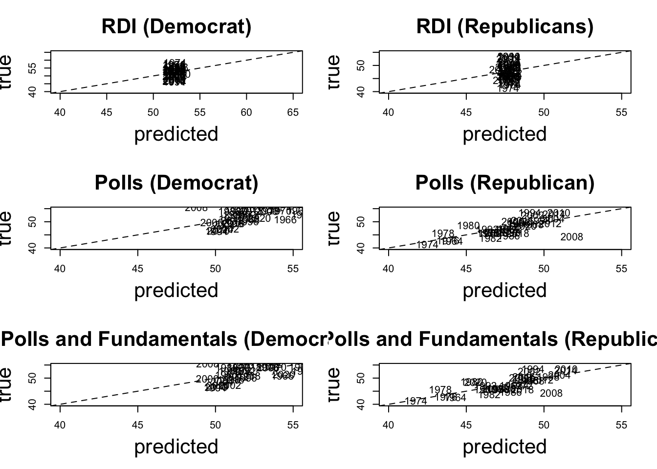
All in all, I selected the polls+fundamentals model as the overall best model due to it’s lower average adjusted r^2 between the two models. Using this model, I aimed to yield an overall forecast of the 2022 election vote percentage for each of the two parties. Overall, my model predicted that the democrats would receive 51.62% of votes while Republicans would receive 48.342% of the votes. Overall, I think the key insight I will draw away from this week is the importance and predictive success of polls in forecasting party vote share. Meanwhile, I believe that I have sufficiently ruled out true economic conditions as a strong predictor once again. Yet, I’m curious if people’s perceptions of the status of the economy are a more predictive measure than the true economic conditions themselves. I’m eager to improve this model next week and look at possibly the effects of President Biden’s tenure in office and incumbency in the midterms.
##        1
## 51.62448
## 1
## 48.34296CITATIONS:
Nate Silver. “How Fivethirtyeight’s House, Senate and Governor Models Work.” FiveThirtyEight, FiveThirtyEight, 12 Sept. 2018, https://fivethirtyeight.com/methodology/how-fivethirtyeights-house-and-senate-models-work/.
G. Elliott Morris. “How the Economist Presidential Forecast Works.” The Economist, The Economist Newspaper, https://projects.economist.com/us-2020-forecast/president/how-this-works.